WavTTS
WavTTS: Towards High-Quality Zero-Shot TTS via Direct Raw Waveform Modeling
WavTTS models raw waveforms directly for zero-shot TTS, avoiding lossy compressed representations. It uses diffusion transformers with multi-scale mel-spectrogram guidance and tailored noise scheduling to deliver high-quality speech synthesis without relying on vocoders or codecs.
Demos
These demos illustrate WavTTS's capability for high-quality zero-shot TTS by directly modeling raw waveforms, avoiding compressed representations. Evaluate the naturalness and clarity in English and Chinese samples, focusing on pronunciation and prosody. The image explains the end-to-end training and inference pipeline using diffusion transformers and mel-spectrogram guidance.

Links
Paper & demos
Code & resources
Impact
Abstract
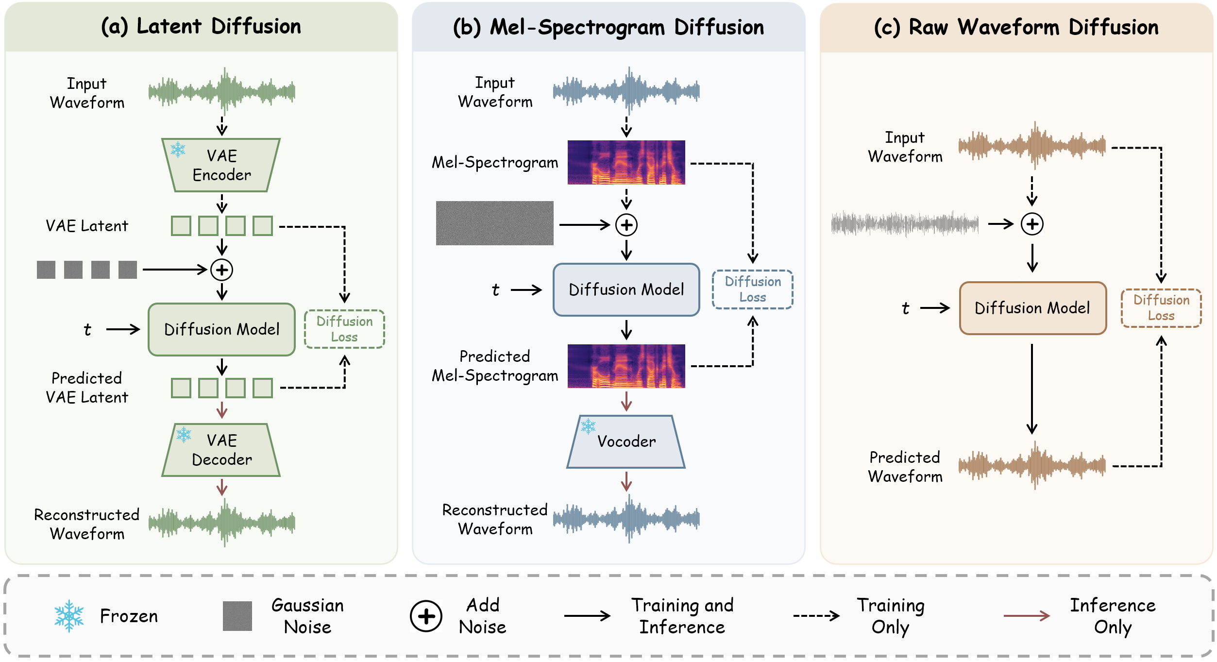
Recently, diffusion models operating on VAE latents or mel-spectrograms have become the dominant paradigm for zero-shot TTS. Although these compressed representations improve generation efficiency, they inevitably suffer from information loss and non-end-to-end training. Theoretically, directly modeling raw waveforms circumvents these issues; however, this direction remains underexplored and is often deemed difficult due to the extremely long sequence length of audio signals. To overcome this, we propose WavTTS, the first raw waveform generative TTS model that substantially narrows the gap with latent-space generative models. Built upon the flow matching with Diffusion Transformer (DiT), WavTTS directly models speech waveforms via a simple patchification strategy, while integrating multi-scale mel-spectrogram supervision to provide perceptual guidance during training. Furthermore, we investigate the impact of prediction targets and noise scheduling in waveform diffusion, and develop an effective schedule design to improve generation quality. Evaluations on open-source benchmarks demonstrate that WavTTS closely approaches the performance of current state-of-the-art latent generative zero-shot TTS models, while substantially outperforming previous end-to-end speech generation models. Our findings demonstrate the feasibility of scaling diffusion-based TTS directly in the waveform space, opening a new direction for end-to-end speech generation.
Introduction and Motivation
WavTTS addresses a central question in modern text-to-speech (TTS): can high-quality zero-shot voice cloning be achieved by generating speech directly in the raw waveform space, rather than in compressed latent spaces or mel-spectrogram space? The paper argues that the dominant non-autoregressive (NAR) diffusion and flow-matching TTS pipelines improve efficiency by operating on reduced acoustic representations, but those representations are inherently lossy and typically require pre-trained autoencoders or vocoders. This creates a multi-stage pipeline with information loss, reconstruction artifacts, and non-end-to-end training.
The authors position WavTTS as a direct response to this gap. The model is a flow-matching TTS system built on a Diffusion Transformer (DiT) backbone that models raw waveforms end-to-end, without relying on neural codecs, mel autoencoders, or vocoders. The key challenge is sequence length: raw audio is extremely long, so a naive waveform diffusion model is difficult to train and sample. WavTTS tackles this with a simple patchification strategy, an $x$-prediction objective, auxiliary multi-scale mel-spectrogram supervision, and noise-aware training/inference schedules tuned specifically for waveform-space generation.
The paper’s core claim is not that waveform modeling is trivially easier than latent modeling, but that it becomes feasible when the diffusion formulation, target parameterization, spectral supervision, and noise schedule are all adapted to the high-dimensional time-domain setting. The reported results show that WavTTS narrows the gap to state-of-the-art latent/mel zero-shot TTS systems, while outperforming prior end-to-end waveform generation baselines by a large margin.
Method Overview

Raw waveform flow matching with an infilling formulation
WavTTS follows the flow-matching view of diffusion as an ordinary differential equation (ODE) that transports Gaussian noise to data. Given clean speech waveform $x_1 \sim p(x_1)$ and noise sample $x_0 \sim \mathcal{N}(0, I)$, the interpolated state is
$$x_t = (1-t)x_0 + t x_1, \quad t \in [0,1].$$
The standard rectified-flow objective learns the velocity field $v_t = x_1 - x_0$ by regression:
$$\mathcal{L}_{\mathrm{FM}} = \mathbb{E}_{t, x_0, x_1} \left[ \| v_\theta(x_t, t) - v_t \|_2^2 \right].$$
Rather than predicting the velocity directly, WavTTS reformulates the problem as clean-waveform prediction. The network outputs $x_\theta = \mathrm{net}_\theta(x_t, t)$ and the FM objective can be rewritten in $x$-prediction form as
$$\mathcal{L}_{\mathrm{FM}} = \mathbb{E}_{t, x_0, x_1} \left[ \left\| \frac{x_\theta - x_1}{1-t} \right\|_2^2 \right].$$
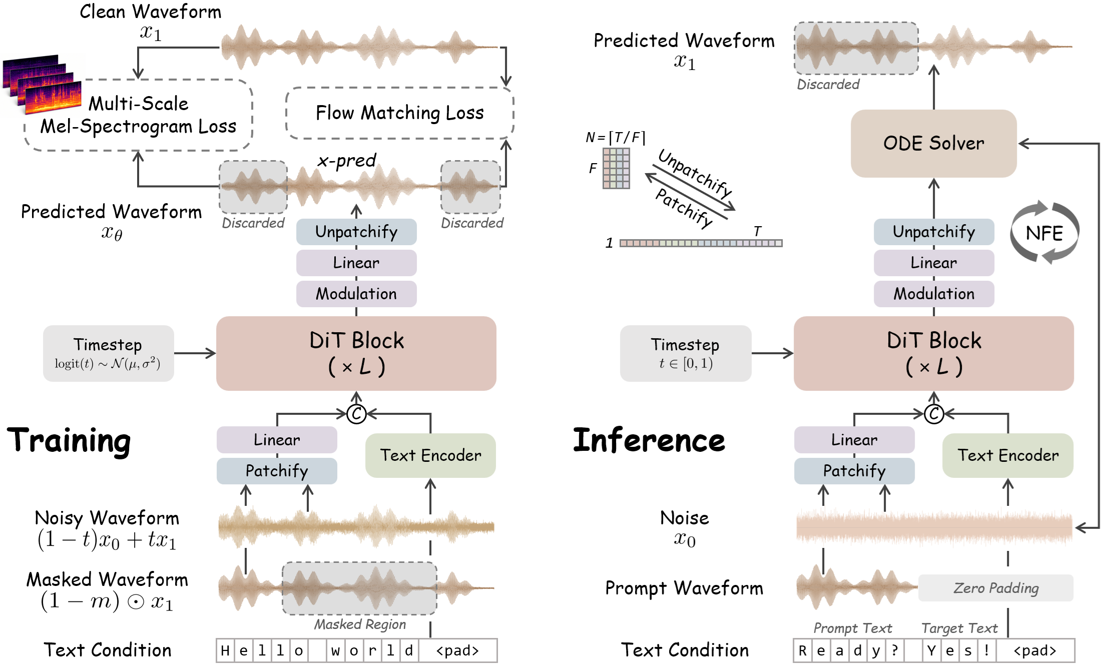
For zero-shot TTS, the model is trained as a text-conditioned speech infilling system in the style of Voicebox. A contiguous mask $m \in \{0,1\}^T$ hides the target region, and the audio prompt is the unmasked context $x_{\mathrm{ctx}} = (1-m) \odot x_1$. The text condition is the full transcript $y$, represented as bilingual pinyin and alphabet tokens. During training, the authors randomly mask a continuous segment covering 70%--100% of the audio prompt, so the model learns to inpaint speech under strong missing-context conditions.
The model uses patchification to shorten the sequence length: the 1D waveform is divided into non-overlapping blocks of length $F=160$, yielding a 100 Hz patch sequence. The patchified noisy waveform and prompt are embedded by two-layer linear projections, and the text sequence is padded with filler tokens to align to the audio-patch length. The text encoder is built from four ConvNeXt V2 blocks, and the text and audio streams are concatenated as input to the DiT backbone. The model then predicts the masked waveform region, which is unpatchified back to the full waveform.
The masked training objective used in the zero-shot setting is
$$\mathcal{L}_{\mathrm{FM}} = \mathbb{E}_{t, x_0, x_1} \left[ \left\| \frac{(x_\theta(x_t, t, x_{\mathrm{ctx}}, y) - x_1) \odot m}{1-t} \right\|_2^2 \right].$$
DiT supplies the backbone computation, with timestep $t$ injected through adaLN-Zero conditioning. The paper also uses RMSNorm and RoPE across Transformer layers. To support classifier-free guidance (CFG), both text and audio prompt are dropped with probability $0.1$ during training, enabling an unconditional branch at inference time.
Inference and classifier-free guidance
At inference, WavTTS uses Euler integration over a discrete time grid $0=t_0<\cdots<t_K=1$. Each step updates the latent waveform estimate by
$$x_{t_{i+1}} = x_{t_i} + (t_{i+1}-t_i) \frac{x_\theta(x_{t_i}, t_i, x_{\mathrm{ctx}}, y) - x_{t_i}}{1-t_i}.$$
CFG is applied by extrapolating conditional and unconditional predictions:
$$\tilde{x}_\theta = x_\theta(x_t, t, x_{\mathrm{ctx}}, y) + \alpha \Big(x_\theta(x_t, t, x_{\mathrm{ctx}}, y) - x_\theta(x_t, t, \emptyset, \emptyset)\Big),$$
where $\alpha$ is the guidance scale. The experimental setup uses $\alpha=3$ and $50$ function evaluations (NFEs). For zero-shot generation, the transcript of the reference audio and the target text are concatenated, and the target duration is estimated from the character-length ratio between the reference and target text. That duration determines the masked region after the prompt audio.
Multi-scale mel-spectrogram supervision
A major design choice is to add a perceptual auxiliary loss on the predicted waveform. The authors note that raw waveform modeling is high-dimensional and contains a great deal of sample-level redundancy. The FM objective alone can waste capacity fitting perceptually unimportant details. To guide the model toward human-relevant structure, WavTTS adds a multi-scale mel-spectrogram loss inspired by vocoder and codec literature.
The mel loss is computed directly on the predicted waveform $x_\theta$ and the ground-truth waveform $x_1$ over the masked region:
$$\mathcal{L}_{\mathrm{mel}} = \mathbb{E}_{t, x_0, x_1} \left[ \sum_{s \in \mathcal{S}} \frac{\left\| m^{(s)} \odot \left( \Phi_s(x_1) - \Phi_s(x_\theta) \right) \right\|_1}{\| m^{(s)} \|_1} \right],$$
and the total objective is
$$\mathcal{L} = \mathcal{L}_{\mathrm{FM}} + \lambda_{\mathrm{mel}}\mathcal{L}_{\mathrm{mel}}.$$
The mel supervision uses seven resolutions with window sizes $[32, 64, 128, 256, 512, 1024, 2048]$ and corresponding mel bins $[5, 10, 20, 40, 80, 160, 320]$. The hop size at each scale is one quarter of the window length. All transforms use magnitude spectrograms, reflective padding, and centered STFT computation. The default weight is $\lambda_{\mathrm{mel}}=0.05$.
Noise-aware waveform-space training and inference
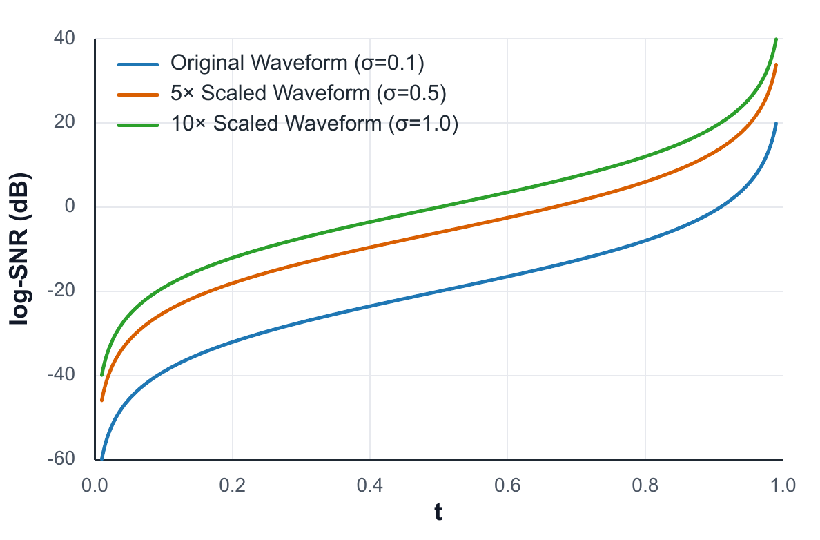
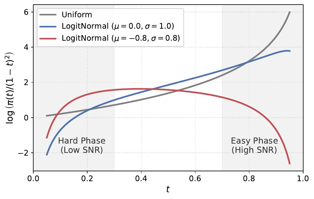
The paper emphasizes that noise design is especially important in waveform space. Raw audio has a much smaller empirical standard deviation than a unit Gaussian prior because speech contains silence and low-energy regions. The authors report approximate waveform standard deviations of about $0.12$ on Emilia and $0.07$ on LibriTTS. This creates a signal-to-noise mismatch along the interpolation path and makes early training timesteps extremely noisy.
To correct the scale mismatch, WavTTS applies Signal-Noise Variance Alignment: the target waveform is scaled as $x_1' = k x_1$ so that its variance is closer to that of the Gaussian prior. The paper derives the log-SNR trajectory as
$$\mathrm{Log\text{-}SNR}(t) = 20 \log_{10}\left(\frac{t}{1-t}\right) + 20 \log_{10}\left(\frac{\sigma_{x_1}}{\sigma_{x_0}}\right),$$
showing that variance mismatch shifts the whole trajectory downward. The default scaling factor is $k=9$, which approximately aligns Emilia’s waveform scale to the noise prior. During inference, the scaled waveform is rescaled back by $1/k$.
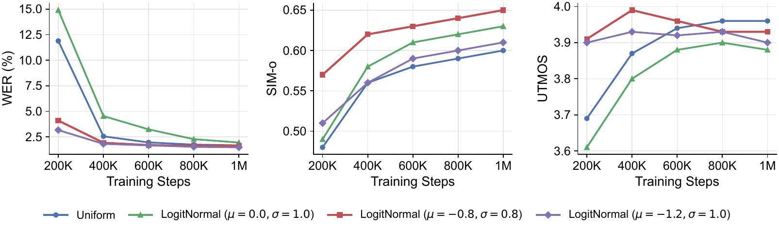
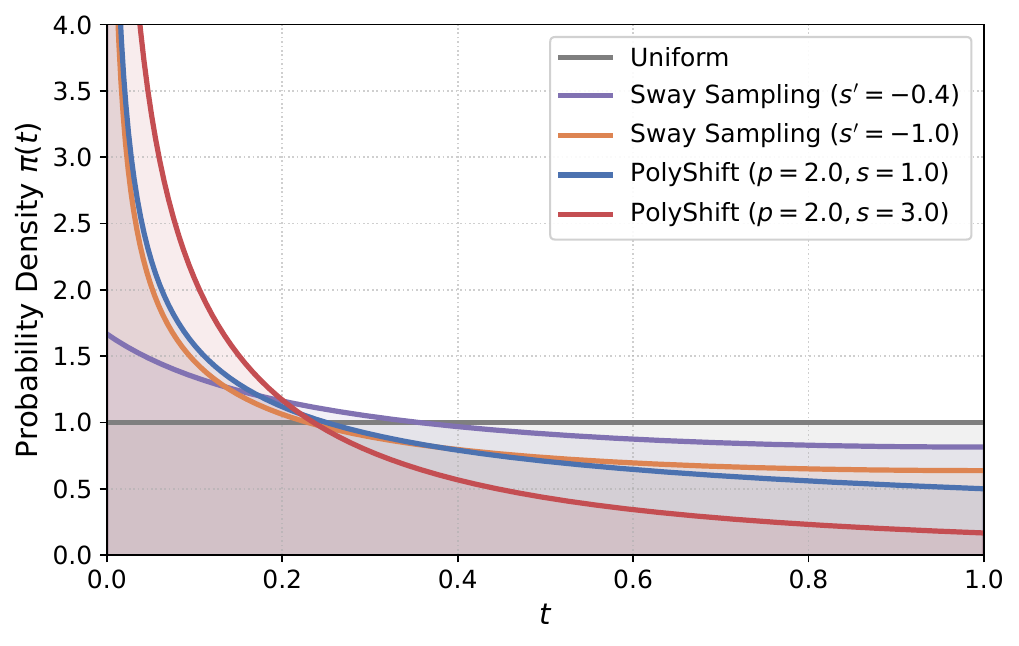
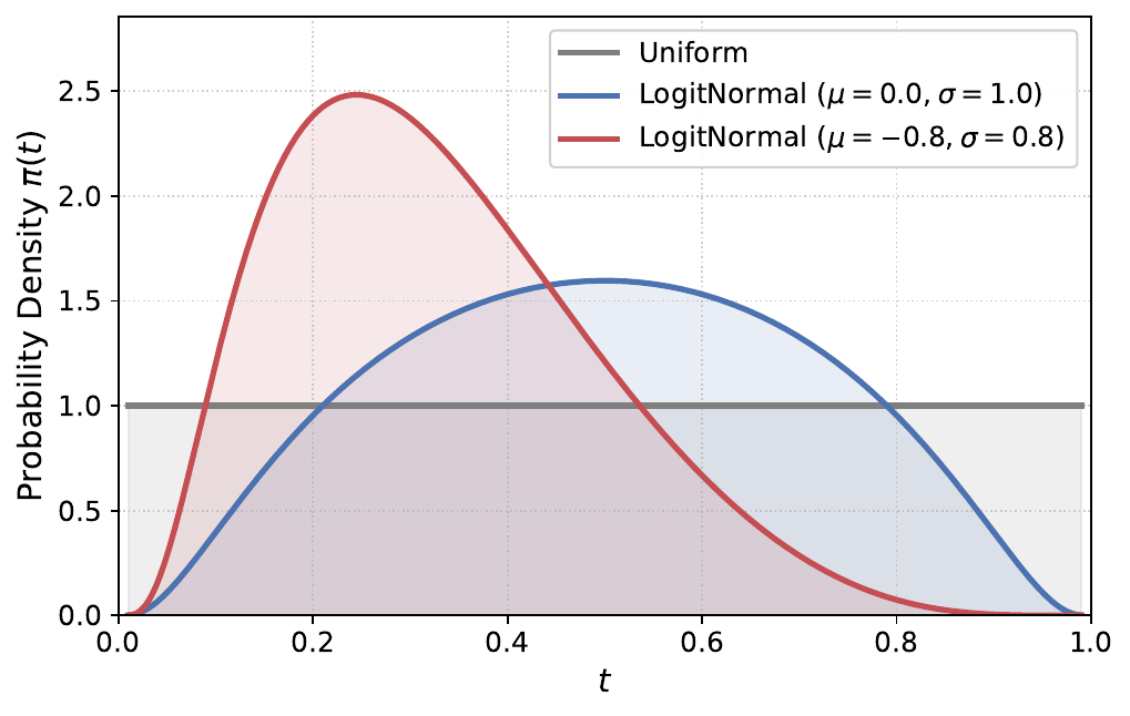
To complement variance alignment, the authors introduce Noise-Shifted Temporal Scheduling. Instead of sampling $t$ uniformly, training timesteps are drawn from a logit-normal distribution $t = \operatorname{sigmoid}(u)$, where $u \sim \mathcal{N}(\mu, \sigma^2)$. Setting $\mu<0$ biases the density toward high-noise regions, which the authors interpret as implicitly upweighting early, low-SNR states. The default schedule uses $\mu=-0.8$ and $\sigma=0.8$. The paper also develops a more aggressive inference-time shift called PolyShift:
$$t = \frac{\tau^p}{\tau^p + s(1-\tau^p)},$$
where $\tau$ is a uniform grid variable, $p$ is a power factor, and $s$ is a shift factor. The default inference schedule uses $p=2$ and $s=3$. In the authors’ interpretation, denser early integration reduces error accumulation in the noisiest part of the ODE trajectory, which is especially important in high-dimensional waveform generation.
Experimental Setup
WavTTS is trained on Emilia, an open-source corpus of approximately 95K hours of English and Chinese speech. For zero-shot evaluation, the paper uses Seed-TTS test-en, which contains 1,088 samples from Common Voice, and Seed-TTS test-zh, which contains 2,020 samples from DiDiSpeech. For standard TTS comparison against prior end-to-end speech generation systems, the paper also evaluates on 682 in-domain LJSpeech test samples and on the LibriSpeech-PC test-clean subset with 1,127 English samples.
The main configuration trains for 1.2M steps on 8 NVIDIA A100 80GB GPUs, with a batch size of 153,600 audio patch frames, corresponding to roughly $0.43$ hours of audio. Optimization uses AdamW with peak learning rate $7.5 \times 10^{-5}$, 20K warmup steps, and then a constant learning rate. Audio is resampled to 16 kHz and patch size is fixed to $F=160$, giving a 100 Hz sequence rate. The default settings are $\lambda_{\mathrm{mel}}=0.05$, scaling factor $k=9$, logit-normal timestep sampling with $\mu=-0.8$ and $\sigma=0.8$, 50 NFEs, CFG scale $\alpha=3$, and PolyShift inference with $p=2$, $s=3$.
The evaluation metrics are all reproducible model-based scores: WER for English intelligibility using Whisper-large-v3, CER for Chinese using Paraformer-zh, SIM-o for speaker similarity using a WavLM-based speaker verification model, and UTMOS for naturalness. The paper compares WavTTS against representative AR systems such as CosyVoice, CosyVoice 2, Llasa, and Spark-TTS; NAR latent/mel systems such as MaskGCT, E2-TTS, F5-TTS, ZipVoice, and LongCat-AudioDiT; and end-to-end waveform systems such as WaveGrad 2, VITS, and JETS.
Main Results
Zero-shot TTS on Seed-TTS
On Seed-TTS test-en and test-zh, WavTTS achieves the strongest English intelligibility and naturalness among the reported systems, while remaining competitive on Chinese. The paper’s key takeaway is that direct waveform modeling can approach the performance of state-of-the-art latent/mel TTS systems, despite using no pre-trained codec or vocoder.
| Model | Params | Data (hrs) | WER ↓ | SIM-o ↑ | UTMOS ↑ | CER ↓ | SIM-o ↑ | UTMOS ↑ |
|---|---|---|---|---|---|---|---|---|
| Ground Truth | -- | -- | 1.79 | 0.73 | 3.53 | 1.25 | 0.75 | 2.78 |
| CosyVoice | 416M | 170K Multi. | 4.29 | 0.61 | -- | 3.63 | 0.72 | -- |
| CosyVoice 2 | 618M | 167K Multi. | 2.57 | 0.65 | -- | 1.45 | 0.75 | -- |
| Llasa-1B | 1370M | 250K Multi. | 3.22 | 0.57 | -- | 1.89 | 0.67 | -- |
| Spark-TTS | 507M | 102K Multi. | 1.98 | 0.58 | -- | 1.20 | 0.67 | -- |
| MaskGCT | 1048M | 100K Emilia | 2.36 | 0.71 | 3.57 | 2.48 | 0.77 | 2.64 |
| E2-TTS | 333M | 100K Emilia | 2.21 | 0.71 | 3.20 | 1.97 | 0.73 | 2.27 |
| F5-TTS | 336M | 100K Emilia | 1.65 | 0.66 | 3.73 | 1.55 | 0.75 | 2.94 |
| ZipVoice | 123M | 100K Emilia | 1.60 | 0.70 | 3.83 | 1.40 | 0.75 | 3.15 |
| LongCat-AudioDiT | 1420M | 100K Multi. | 1.94 | 0.76 | 3.80 | 1.10 | 0.81 | 3.16 |
| WavTTS | 673M | 100K Emilia | 1.50 | 0.65 | 3.92 | 1.59 | 0.73 | 3.08 |
Compared with the strongest baselines, WavTTS achieves the best English WER and UTMOS. Its WER of $1.50\%$ beats ZipVoice ($1.60\%$) and F5-TTS ($1.65\%$), and its UTMOS of $3.92$ is the best in the table. On speaker similarity, however, WavTTS trails the best latent-model systems, especially LongCat-AudioDiT, which reaches SIM-o $0.76$ on English and $0.81$ on Chinese. The authors attribute this to the difficulty of prioritizing target-speaker timbre when generating high-dimensional raw waveforms that also encode phase, ambience, and fine acoustic detail.
Comparison with end-to-end waveform generation systems
To compare against prior end-to-end speech generation work, the paper evaluates on LJSpeech and LibriSpeech-PC. For a fairer naturalness comparison, WavTTS is prompted with a fixed audio clip randomly selected from LJSpeech. The results show that WavTTS matches or exceeds supervised waveform generators, even under a zero-shot setup.
| Model | LJSpeech WER ↓ | LJSpeech UTMOS ↑ | LibriSpeech-PC WER ↓ | LibriSpeech-PC UTMOS ↑ |
|---|---|---|---|---|
| Ground Truth | 3.42 | 4.36 | 2.23 | 4.10 |
| WaveGrad 2 | 25.19 | 3.24 | 33.77 | 3.05 |
| VITSVCTK | 9.34 | 4.06 | 10.23 | 4.03 |
| VITSLJ | 3.72 | 4.37 | 2.23 | 4.36 |
| JETS | 3.73 | 4.36 | 3.00 | 4.34 |
| WavTTS | 3.43 | 4.39 | 2.02 | 4.36 |
WavTTS obtains the best WER and UTMOS on both datasets. Notably, it slightly outperforms ground truth on the UTMOS metric for LJSpeech and matches the best UTMOS on LibriSpeech-PC, while also achieving the lowest WER on both sets. The paper emphasizes that this is notable because many prior end-to-end systems, including VITS and JETS, still rely on intermediate latent representations or adversarial decoders rather than direct raw-waveform generation.
Why raw waveform modeling can work
The paper’s comparative analysis suggests that raw-waveform modeling is viable because the combination of patchification, $x$-prediction, mel supervision, and carefully designed noise schedules makes optimization tractable. In other words, the main challenge is not the waveform space itself but the mismatch between naive diffusion training and waveform statistics. Once the model and schedules are aligned with the data distribution, direct waveform generation becomes competitive with compressed representations.
Comparison of Acoustic Representations
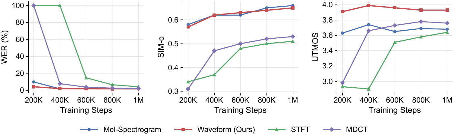
The appendix compares raw waveform modeling with other time-frequency representations under the same flow-matching backbone. For fairness, the STFT and MDCT systems use the same DiT backbone as the 673M waveform model, the same $x$-prediction objective, and no auxiliary mel loss. The only change is the acoustic representation.
For STFT-based modeling, the paper extracts 402-dimensional features by splitting real and imaginary parts of the complex coefficients; the transform uses a Hann window, FFT size 400, and hop length 160, yielding a 100 Hz frame rate. The coefficients already have a scale close to unit variance, so no extra scaling is applied. For MDCT, the transform uses a 320-sample Vorbis window and 160-hop overlap, producing 160-dimensional feature vectors. Because MDCT coefficients have a much smaller standard deviation, the paper multiplies them by $200$ before flow matching.
The qualitative conclusion is that waveform and mel-spectrogram models both converge efficiently and reach useful performance by around 200K steps, but waveform modeling yields faster early intelligibility convergence and better final naturalness. Specifically, at 200K steps the waveform model reaches $4.10\%$ WER versus $9.76\%$ for mel-spectrogram modeling, and at 1M steps it attains UTMOS $3.93$ versus $3.68$ for mel-spectrograms, with similar speaker similarity. By contrast, STFT and MDCT converge much more slowly: the MDCT model starts producing recognizable speech around 400K steps, while STFT requires around 600K steps. The paper suggests this is because STFT requires modeling complex-valued magnitude-phase structure and MDCT exhibits a sharply peaked distribution with outliers that are less friendly to flow matching.
Ablations and Analysis
Prediction target and mel-loss weight
The first ablation asks whether $x$-prediction is better than velocity prediction, and how much mel supervision is optimal. All variants are trained for 1M steps on 8 A100 GPUs and evaluated on Seed-TTS test-en with the same inference strategy.
| Prediction target | $\lambda_{\mathrm{mel}}$ | WER ↓ | SIM-o ↑ | UTMOS ↑ |
|---|---|---|---|---|
| v-prediction | 0.05 | 1.67 | 0.61 | 3.94 |
| x-prediction | 0 | 1.92 | 0.56 | 3.77 |
| x-prediction | 0.01 | 1.77 | 0.60 | 3.87 |
| x-prediction | 0.05 | 1.65 | 0.65 | 3.93 |
| x-prediction | 0.2 | 1.74 | 0.60 | 3.89 |
| x-prediction | 0.5 | 1.81 | 0.55 | 3.82 |
The paper concludes that $x$-prediction is the better target for waveform modeling because it directly predicts the clean signal rather than the noisy velocity field. Compared with $v$-prediction, $x$-prediction yields slightly better intelligibility and a clear improvement in speaker similarity. The mel loss is essential: removing it causes a broad degradation across all metrics, and the paper reports that convergence is much slower without spectral supervision. Overweighting the mel term also hurts performance, suggesting that too much perceptual loss can distract the model from learning a clean waveform-space flow. The chosen default, $\lambda_{\mathrm{mel}}=0.05$, is the best trade-off.
Waveform scaling and signal-noise variance alignment
The scaling ablation tests the waveform scaling factor $k$ used to align waveform variance with the noise prior.
| $k$ | WER ↓ | SIM-o ↑ | UTMOS ↑ |
|---|---|---|---|
| 1 | 4.18 | 0.32 | 2.40 |
| 5 | 1.51 | 0.59 | 3.81 |
| 9 | 1.65 | 0.65 | 3.93 |
| 10 | 1.82 | 0.64 | 3.87 |
Without scaling ($k=1$), performance collapses, especially on SIM-o and UTMOS, confirming that the raw waveform scale is too small relative to the unit Gaussian prior. The paper interprets this as the model spending too much of the diffusion trajectory in an extremely low-SNR regime. Scaling improves all metrics dramatically, with $k=9$ chosen as the default because it gives the best speaker similarity and naturalness. A smaller scale such as $k=5$ slightly improves WER but introduces audible artifacts such as electronic noise and incomplete denoising, according to subjective listening. This is an important point: the best intelligibility score is not always the best overall perceptual result.
Training and inference timestep schedules
The paper then studies noise-shifted schedules during training and inference. During training, a logit-normal sampling distribution with negative $\mu$ concentrates more probability mass in the high-noise regime. The authors show that this accelerates early convergence and improves final WER, but if the shift becomes too aggressive, speaker similarity and naturalness start to degrade. Uniform sampling converges more slowly but can achieve slightly higher final UTMOS because it spends more time refining low-noise details.
| Inference schedule | WER ↓ | SIM-o ↑ | UTMOS ↑ |
|---|---|---|---|
| Uniform | 1.78 | 0.63 | 3.77 |
| Sway Sampling ($s'=-1.0$) | 1.68 | 0.64 | 3.88 |
| PolyShift ($p=2.0, s=1.0$) | 1.60 | 0.64 | 3.88 |
| PolyShift ($p=2.0, s=3.0$) | 1.65 | 0.65 | 3.93 |
| PolyShift ($p=2.0, s=5.0$) | 1.58 | 0.65 | 3.92 |
For inference, noise-shifted schedules outperform uniform sampling. Sway Sampling already improves over uniform, and the proposed PolyShift gives further gains by allowing more flexible allocation of steps to the early, noisy region. The default PolyShift setting $p=2$, $s=3$ is selected because it provides the best balance between SIM-o and UTMOS. A more aggressive shift, $s=5$, slightly lowers WER but produces more noticeable background noise in subjective listening. The paper therefore treats early denoising as a delicate trade-off: too little early emphasis slows convergence, but too much can harm later-stage refinement.
Scaling behavior with data and model size
The scaling experiments use a smaller 340M-parameter model and the full 673M model on two datasets: LibriTTS, which is about 585 hours and represents a low-resource regime, and Emilia, which is about 100K hours and is much larger and more diverse. The main conclusion is that both data scale and model scale matter, but model scaling only helps when the training data is sufficiently large.
| Training data | Model size | WER ↓ | SIM-o ↑ | UTMOS ↑ |
|---|---|---|---|---|
| LibriTTS (585 hrs) | 340M | 2.16 | 0.35 | 3.95 |
| LibriTTS (585 hrs) | 673M | 2.12 | 0.31 | 3.94 |
| Emilia (100K hrs) | 340M | 1.74 | 0.56 | 3.87 |
| Emilia (100K hrs) | 673M | 1.65 | 0.65 | 3.93 |
On LibriTTS, both models generalize poorly to out-of-domain zero-shot evaluation and achieve SIM-o values only in the $0.3$ range. On Emilia, performance improves sharply: WER drops below $2\%$ and speaker similarity rises substantially. Increasing model size from 340M to 673M helps on Emilia, especially on SIM-o, but offers little benefit on the smaller LibriTTS regime. The takeaway is that waveform-space generative modeling is data-hungry, and its scaling behavior follows the same broad pattern seen in other large-scale TTS systems: capacity helps, but only when matched with enough data.
Discussion and Limitations
The paper does not present a separate formal limitations section, but several constraints are clearly acknowledged in the experiments and discussion. First, speaker similarity remains behind the strongest latent-space baselines, even though WavTTS is competitive on intelligibility and naturalness. This suggests that waveform-space generation still has room to improve in speaker-oriented control or alignment. Second, the waveform space is more sensitive to noise scheduling than compressed representations: overly weak variance alignment or overly aggressive temporal shifting can lead to background noise, electronic artifacts, or incomplete denoising.
Third, the scaling results show that small-data waveform modeling is weak, and that larger models do not automatically help unless the dataset is sufficiently large and diverse. Fourth, the comparison with STFT and MDCT suggests that not all lossless or nearly lossless acoustic representations are equally friendly to flow matching; direct waveform modeling was the simplest and most effective among the representations tested, while STFT and MDCT required more steps and showed slower convergence. The authors explicitly suggest future work on dynamic timestep scheduling that changes the training distribution over the course of optimization, which could improve the balance between coarse structure learning and fine acoustic refinement.
Overall, the paper’s message is that raw waveform generation is feasible, but only with careful attention to the geometry of the noise path and the perceptual objectives. WavTTS does not eliminate the challenges of waveform-space generation; rather, it demonstrates that those challenges can be managed well enough to reach the neighborhood of state-of-the-art zero-shot TTS quality.
Bottom-Line Takeaway
WavTTS is a strong proof-of-concept for direct, end-to-end raw-waveform zero-shot TTS. Its contribution is not just replacing mel or latent representations with waveform samples, but showing that waveform-space flow matching becomes practical when combined with patchification, $x$-prediction, multi-scale mel supervision, variance alignment, and noise-shifted schedules. The resulting system achieves the best English WER and UTMOS on Seed-TTS among the reported baselines, matches or exceeds prior end-to-end waveform systems on standard TTS benchmarks, and makes a compelling case that raw-waveform diffusion is a viable future direction for high-quality speech synthesis.
Code & Implementation
This repository implements the WavTTS framework presented in the paper, targeting end-to-end zero-shot text-to-speech synthesis directly in the raw waveform domain.
The core WavTTS model code is organized under the src/wavtts/ directory. Key components include:
model/: Implementation of the core model (CFM) and related modules, dataset handling, and training utilities. Thetrainer.pyscript encapsulates the training loop and optimization strategy, consistent with the paper's description of training with flow matching and diffusion transformer approaches.infer/: Contains scripts and utilities for performing zero-shot inference using the WavTTS model. This includes a command-line interface (infer_cli.py) that enables generating speech waveforms directly from text inputs and a reference audio prompt, showcasing the zero-shot capability.configs/: Configuration files (e.g.,WavTTS.yaml) define model and training hyperparameters, aligning with experimental setups in the paper.train/: Training entry points and dataset preparation scripts, supporting reproducibility of results and enabling training on datasets like Emilia as described in the README.
The repository supports training with advanced distributed training tools (Accelerate), EMA model tracking, and logging integration with WandB or Tensorboard, facilitating model development and evaluation.
Overall, the codebase provides a comprehensive implementation of the WavTTS framework's methodology — direct modeling of raw waveform speech synthesis via diffusion transformers with multi-scale mel spectrogram supervision — and includes end-to-end training and inference workflows as detailed in the paper.