Sparse Autoencoder Steering for TTS
Interpreting and Steering a Text-to-Speech Language Model with Sparse Autoencoders
The paper uses sparse autoencoders to interpret and control features in a text-to-speech language model's shared text-speech representation. This enables causal steering of speech attributes such as laughter, speaker gender, and speech rate without altering the spoken content.
Links
Paper & demos
Impact
Abstract
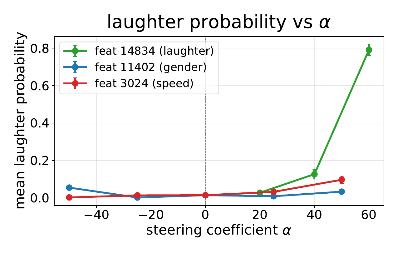
Language models increasingly serve as the backbone of text-to-speech (TTS) systems, yet we understand little about the representations they build when text and generated speech tokens share a single residual stream. We train BatchTopK sparse autoencoders on the LM backbone of CosyVoice3 and introduce a modality-aware auto-interp pipeline that labels each feature from where it fires-text-prefix context, 1-second speech clips, or both. The recovered features are interpretable, spanning phonemes, laughter, accent prompts and speaker gender. Steering through the SAE latent space shows these features are causal rather than merely descriptive: targeted interventions raise laughter probability from 0.02 to 0.79, flip perceived speaker gender, and control speech rate while preserving spoken content. SAE features thus serve both as interpretability objects and as control directions for TTS synthesis.
Overview and main claims
This paper studies mechanistic interpretability for a text-to-speech (TTS) language model backbone, rather than for a text-only LLM. The core setting is CosyVoice3, whose LM backbone processes a mixed sequence containing a text/instruction prefix followed by autoregressively generated discrete speech tokens. The authors ask what sparse autoencoder (SAE) features recover from that shared residual stream, how those features differ by token modality, and whether the recovered features can be used as causal steering directions for speech generation.
The paper’s main claim is that BatchTopK SAEs trained on CosyVoice3 recover interpretable text-modal, audio-modal, and mixed features, and that some of these features are not merely descriptive: latent interventions on the SAE coordinates can materially control perceptual properties of generated speech, including laughter, speaker-gender cues, and speech rate, while preserving spoken content.
At a high level, the paper contributes three things: (1) SAE training on a TTS LM backbone at scale, (2) a modality-aware auto-interpretation pipeline adapted to the mixed text-speech sequence, and (3) a layer-wise analysis showing how feature modality shifts across depth.
Model, data, and SAE training setup
The target model is CosyVoice3, whose LM backbone is Qwen2.5-0.5B with hidden size $896$ and $28$ layers. The backbone receives a text prompt tokenized with BPE and generates $25$ Hz discrete speech tokens autoregressively. The authors attach SAEs to the residual stream of this backbone at multiple layers.
Training uses BatchTopK SAEs with dictionary size $d = 16{,}384$ and $k = 50$ active features per token. The training corpus is approximately $250$ million tokens from the Emilia dataset. The paper states that the SAE objective is the standard reconstruction-plus-sparsity loss with an auxiliary dead-feature loss.
The analysis uses the full layer sweep for modality and reconstruction studies, while layer $20$ is used for most qualitative examples and the steering case studies.
| Component | Reported setting |
|---|---|
| Backbone | Qwen2.5-0.5B inside CosyVoice3 |
| Hidden size / layers | $896$ / $28$ |
| Speech token rate | $25$ Hz |
| SAE dictionary size | $16{,}384$ |
| Active features per token | $k = 50$ |
| Training data | Approximately $250$M tokens from Emilia |
Modality-aware interpretation pipeline
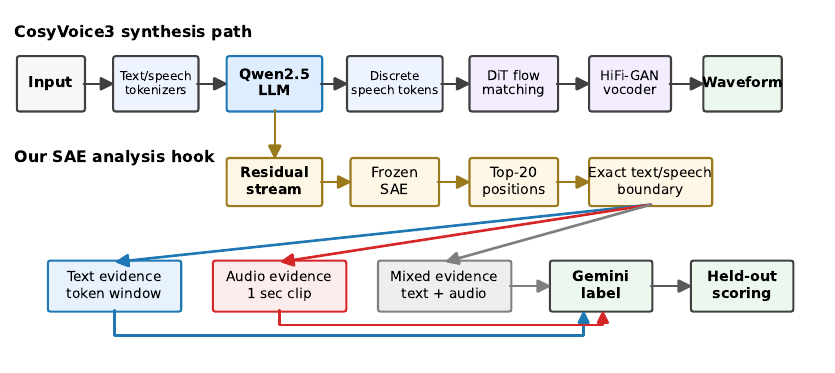
The paper’s interpretation pipeline is designed around a key complication: CosyVoice3 interleaves text prefix tokens and speech tokens in a single residual stream. That means a feature may activate on text-prefix context, on generated speech, or on both. Rather than forcing all evidence into a single format, the pipeline uses the exact token boundaries in each sequence to route the strongest activations to modality-specific evidence.
For each SAE feature, the authors collect the top-20 activating token positions across the dataset by encoding residual-stream activations through the frozen SAE. They use teacher forcing with the sequence layout $[\mathrm{sos} \mid \mathrm{instruct} \mid \mathrm{text} \mid \mathrm{task} \mid \mathrm{speech}]$, where the task token marks the text-to-speech transition. For speech positions, token indices are mapped to timestamps using the $25$ Hz rate, and the source audio is cropped to a $1$-second window centered on the peak position. Padded positions are masked before ranking and extraction.
Feature modality is determined from the composition of the top-20 activations. Let the speech-start position for example $i$ be $b_i$, computed from the prefix lengths and the task marker. A top activation at position $p$ is counted as speech if $p \ge b_i$ and is within the valid sequence length. The speech fraction is then the proportion of the top-20 activations that fall in the speech segment.
The modality thresholds are explicit: features are labeled audio-modal if their speech fraction is at least $0.8$, text-modal if it is at most $0.2$, and mixed otherwise. The paper emphasizes that this is necessary because absolute position is not semantically stable in randomly interleaved text/speech sequences.
Automatic labeling and held-out scoring
The authors adapt LLM-based auto-interpretation to this mixed-modality setting. They use Gemini 3.0 Pro as the labeler, with prompts that differ by feature modality:
- Text-modal features are shown text evidence only: marked token context, activation value, and source text context.
- Audio-modal features are shown only $1$-second speech clips centered on activating speech tokens.
- Mixed features are shown both text evidence and speech clips, and are only labeled when both evidence types are present.
The prompt asks for a single concise sentence describing the property consistently associated with the evidence. For text features, the label may describe lexical, punctuation, language, prompt-style, or transcript properties; for audio features, it may describe acoustic, phonetic, or prosodic properties; for mixed features, it may describe a cross-modal relation if one is visible.
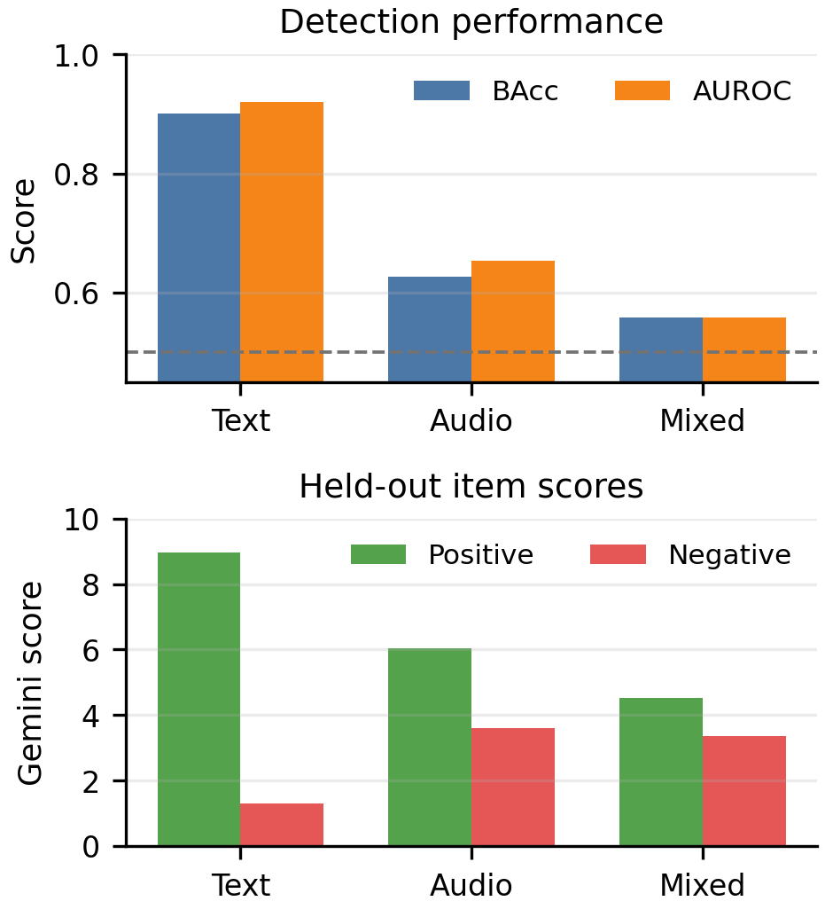
To evaluate label quality, the paper uses a detection-style protocol adapted from prior auto-interp work. Given a proposed label, a held-out scorer rates positive and negative evidence items for how well they match the label. The evaluation reports AUROC and balanced accuracy. To reduce leakage from label-writing examples, the authors use a rank-held-out split: the five strongest activations are reserved for labeling and lower-ranked activations are used for scoring.
For the layer-20 comparison, the paper evaluates all $668$ mixed features together with matched $668$-feature samples of text-modal and audio-modal features. This is the primary quantitative benchmark for auto-interpretation quality in the paper.
Layer-wise reconstruction and modality dynamics
The layer sweep shows that the SAE remains a strong reconstruction model across the backbone, but the feature dictionary changes its modality composition substantially with depth. The most important qualitative pattern is that early and middle layers are multimodal and mixed, late layers become strongly audio-heavy, and the final hidden state reverts to a mostly text-modal subspace.
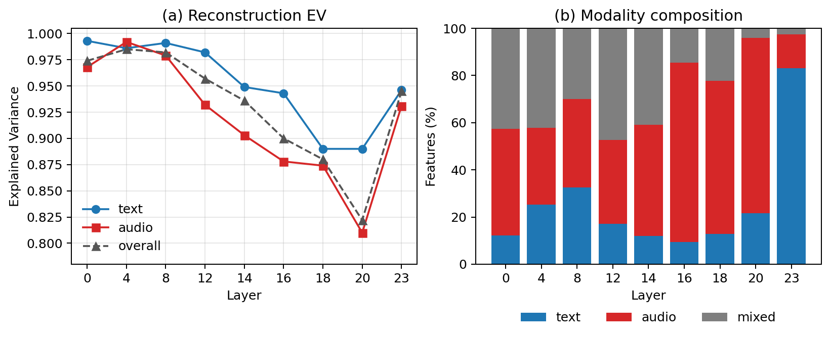
The appendix gives concrete modality proportions across depth. At layer $0$, the dictionary is already strongly multimodal: $12.3\%$ text-modal, $45.1\%$ audio-modal, and $42.6\%$ mixed. Mixed features peak at layer $12$ with $47.3\%$. The late layers form an “audio-commitment zone”: audio-modal features dominate at layer $16$ ($76.1\%$), layer $18$ ($65.0\%$), and layer $20$ ($74.3\%$), while mixed features collapse to $4.1\%$ by layer $20$. Layer $23$, the final hidden state, sharply flips back to a text-dominant composition: $83.1\%$ text-modal, $14.3\%$ audio-modal, and $2.6\%$ mixed.
The paper also reports per-token explained variance on a $5{,}000$-sample sweep. Reconstruction quality is very high in early layers, with overall explained variance around $0.97$--$0.99$ at layers $0$--$8$, then declines through the body of the network to a minimum of $0.82$ at layer $20$. The final layer rebounds to $0.945$. Text positions are generally reconstructed at least as well as audio positions, with the largest text-audio gap at the audio-commitment layers.
This layer-wise pattern is one of the central mechanistic findings of the paper: the shared residual stream does not merely preserve the prefix text, but gradually develops sparse directions that are tied to the generated speech-token stream as acoustic prediction is formed.
| Layer | Text-modal | Audio-modal | Mixed | Notable observation |
|---|---|---|---|---|
| 0 | 12.3% | 45.1% | 42.6% | Already strongly multimodal |
| 12 | Not stated explicitly | Not stated explicitly | 47.3% | Mixed features peak |
| 16 | Minority | 76.1% | Declining | Audio-commitment zone begins |
| 18 | Minority | 65.0% | Declining | Audio remains dominant |
| 20 | Minority | 74.3% | 4.1% | Audio-heavy, mixed nearly gone |
| 23 | 83.1% | 14.3% | 2.6% | Final hidden state reverts to text-modal |
Auto-interpretation quality
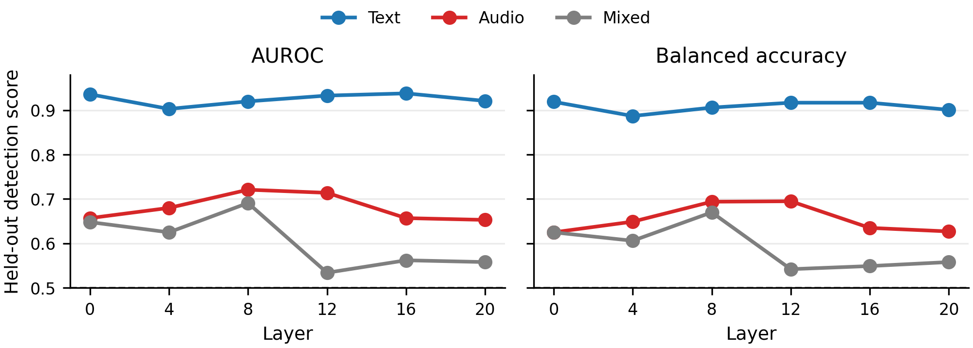
The held-out detection-style evaluation confirms that the modality-aware labeling protocol works best for text features, reasonably well for audio features, and least well for mixed features. For layer $20$, the reported AUROC values are $0.921$ for text-modal labels, $0.653$ for audio-modal labels, and $0.558$ for mixed labels.
The layer-wise appendix reports the same ordering throughout the network. Text-modal labels are consistently easiest to verify, with AUROC roughly in the $0.90$--$0.94$ range. Audio-modal labels are weaker but remain above chance, around $0.65$--$0.72$. Mixed labels are the hardest and most variable, ranging roughly from $0.53$ to $0.69$.
This is an important practical conclusion: single-modality features are often well described by one concise sentence, while mixed features more often combine several correlated textual and acoustic properties and are therefore harder to summarize cleanly.
| Setting | AUROC | Interpretation |
|---|---|---|
| Layer 20, text-modal | 0.921 | Easiest to verify |
| Layer 20, audio-modal | 0.653 | Above chance, but weaker |
| Layer 20, mixed | 0.558 | Hardest in aggregate |
Representative SAE features
The paper’s qualitative examples show that the dictionary learns a mix of very local linguistic features and speech-acoustic features. Text-modal features often correspond to individual tokens, words, years, punctuation, or prompt-side descriptors of voice style and accent. Audio-modal features often correspond to phonemes, short phoneme sequences, laughter, breathing, stuttering, or accent cues. Mixed features sometimes connect the same word or phoneme-like event across both text and speech.
Examples from the appendix include a text feature for the word “British” in speaker-accent descriptions, an audio feature for human laughter, and a mixed feature for the phoneme sequence /ohl/ in both text and speech. Another representative set includes text features for the substring “ang”, the adjective “shrill”, and four-digit years; audio features for /k/, /if/ or /ef/, /ing/, screaming/shouting/heavy breathing, and a mixed feature for stutters, false starts, and hesitation markers.
| Feature | Modality | Auto-interp label | BAcc | AUROC |
|---|---|---|---|---|
| 1376 | Text | Word “British” in speaker-accent descriptions | 1.000 | 1.000 |
| 233 | Audio | The sound of human laughter | 0.750 | 0.750 |
| 5543 | Mixed | The phoneme sequence /ohl/ in text and speech | 0.917 | 0.979 |
Probe-based feature analysis
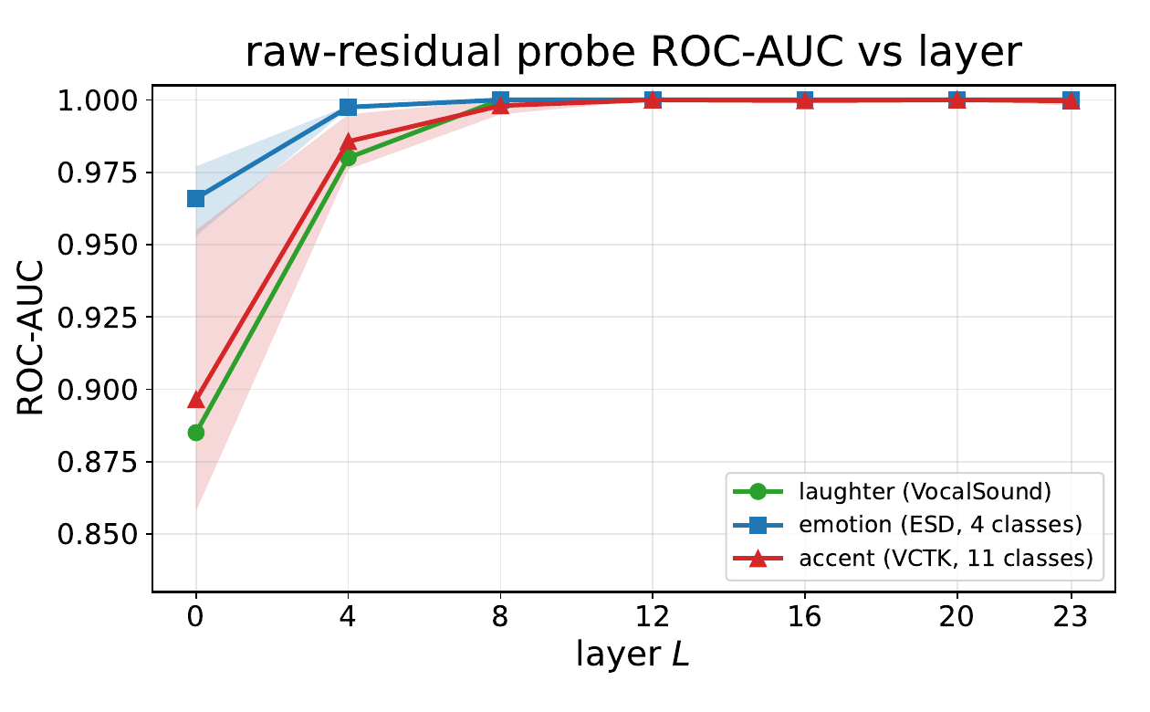
Beyond auto-interpretation, the paper asks whether individual concepts are linearly decodable from the residual stream and whether those concepts are concentrated in SAE coordinates. The authors train binary logistic-regression probes for three speech-style concepts: laughter, emotion, and accent. Probes are evaluated on either the raw residual vector $h_L$ or the SAE latent vector $z_L = \mathrm{SAE}_L(h_L)$, with ROC-AUC reported under stratified $5$-fold cross-validation.
For all three concepts, raw-residual probes become nearly perfect very early in the network. In the layer-wise table, laughter reaches ROC-AUC $0.980$ by layer $4$ and $1.000$ by layer $8$; the emotion and accent probes likewise reach approximately perfect decodability by layer $8$. SAE-latent probes closely track raw-residual probes from around layer $8$, which the authors interpret as evidence that the sparse code preserves the relevant speech-style information while expressing it in dictionary coordinates.
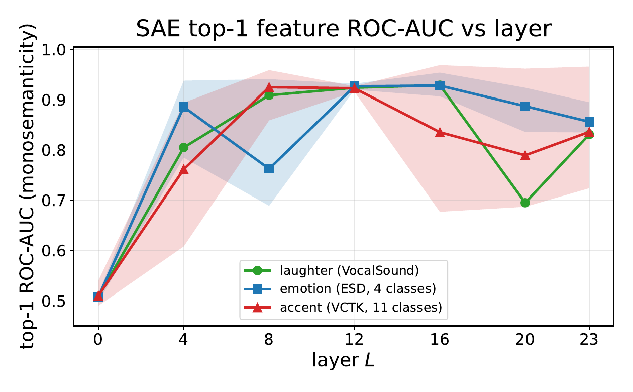
The top-1 SAE analysis is the monosemanticity test: it keeps only the single SAE coordinate with the largest mean absolute probe coefficient and asks how much concept signal remains. The reported top-1 AUCs are below 0.6 at layer $0$, but rise sharply in the middle layers. Laughter peaks around layers $12$--$16$ at $0.924$--$0.929$, emotion peaks around layers $12$--$16$ at $0.927$--$0.928$, and accent is most localized around layers $8$--$12$ with AUC about $0.923$--$0.925$.
| Concept / representation | L0 | L4 | L8 | L12 | L16 | L20 | L23 |
|---|---|---|---|---|---|---|---|
| Laughter, raw residual | 0.885 | 0.980 | 1.000 | 1.000 | 1.000 | 1.000 | 1.000 |
| Laughter, SAE latent | 0.866 | 0.948 | 0.998 | 1.000 | 1.000 | 1.000 | 0.999 |
| Emotion, raw residual mean | 0.966 | 0.998 | 1.000 | 1.000 | 1.000 | 1.000 | 1.000 |
| Accent, raw residual mean | 0.896 | 0.986 | 0.998 | 1.000 | 1.000 | 1.000 | 1.000 |
| Concept | L0 | L4 | L8 | L12 | L16 | L20 | L23 |
|---|---|---|---|---|---|---|---|
| Laughter | 0.508 | 0.805 | 0.909 | 0.924 | 0.929 | 0.695 | 0.831 |
| Emotion mean | 0.507 | 0.886 | 0.763 | 0.927 | 0.928 | 0.887 | 0.856 |
| Accent mean | 0.510 | 0.762 | 0.925 | 0.923 | 0.835 | 0.789 | 0.836 |
The probing experiments are used in the paper as a bridge from interpretability to steering: they identify SAE features whose activations are predictive of controllable speech properties and suggest that some of these properties are concentrated enough to be manipulated through a small number of SAE coordinates.
Steering in SAE latent space
The paper’s causal test is to intervene on SAE coordinates during generation instead of adding a raw residual vector directly. For a hooked residual vector $h$, the authors compute SAE activations
$$ z = \sigma(W_{\mathrm{enc}} h + b_{\mathrm{enc}}) $$
then perturb selected coordinates with
$$ z' = z + \alpha \cdot s \odot \bar{Z}, $$
where $\alpha$ is the steering strength, $s$ is a sparse sign vector controlling polarity, and $\bar{Z}$ provides feature-wise activation scales. The modified latent vector is decoded back to residual space as
$$ \hat{h}' = W_{\mathrm{dec}} z' + b_{\mathrm{dec}}. $$
The hook is applied only to speech-token positions. During prefill it affects the speech-prompt segment; during autoregressive decoding it affects only the current generated speech token. Instruction, text-prefix, and task-token positions are left untouched.
| Feature | Auto-interp label | Reported steering effect |
|---|---|---|
| 14834 | Laughter-like vocal events | More laughter |
| 11402 | Speaker-gender cues | Male/female shift |
| 3024 | Speech-rate variation | Slower/faster speech |

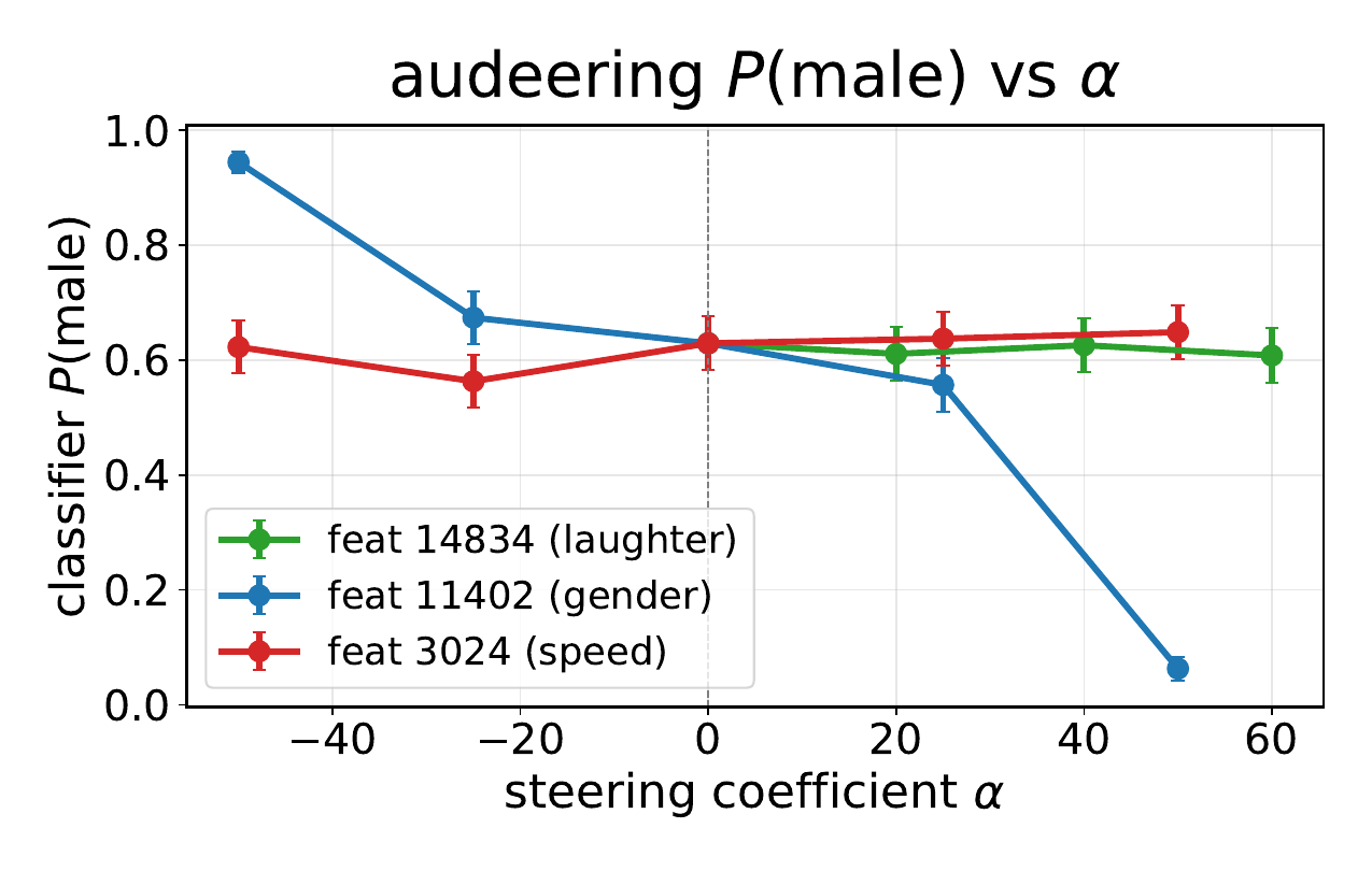
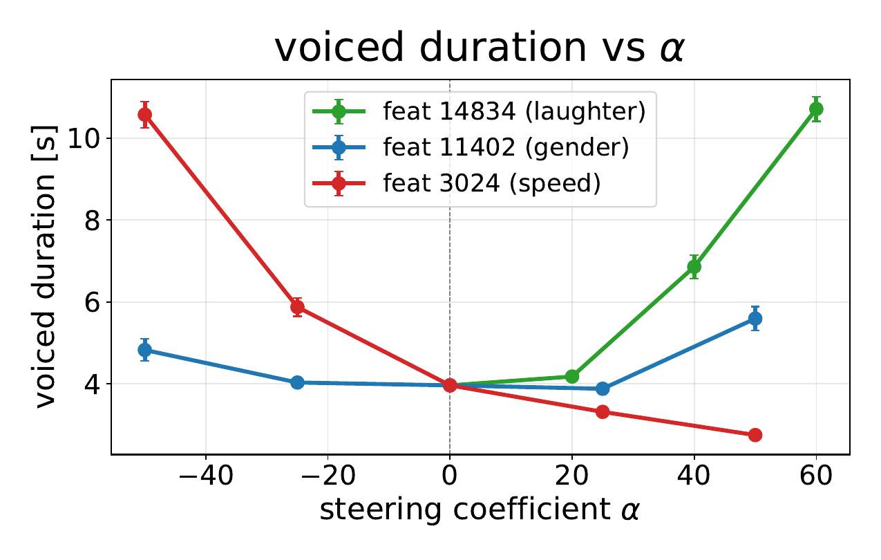
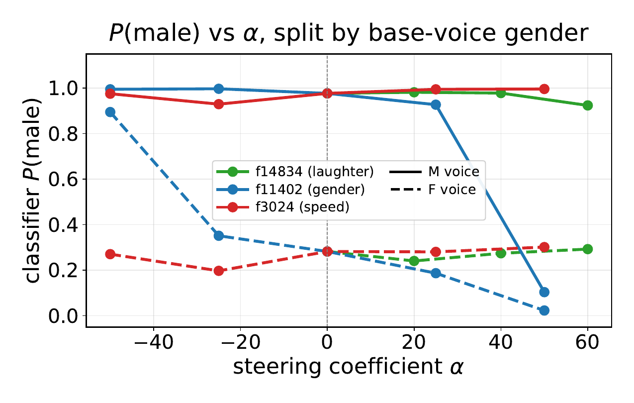
The steering results are strong and specific. Feature $14834$ increases laughter probability from $0.015$ to $0.791$ at $\alpha = +60$. Feature $11402$ changes speaker-gender cues, moving wav2vec2 $P(\mathrm{male})$ from $0.629$ at baseline to $0.944$ at $\alpha = -50$ and $0.063$ at $\alpha = +50$. Feature $3024$ controls speech rate, changing voiced duration from $3.96$ s at baseline to $10.57$ s at $\alpha = -50$ and $2.75$ s at $\alpha = +50$, while preserving spoken content.
The gender plot also breaks the result down by the prompt speaker’s original gender, showing that feature $11402$ shifts both male- and female-prompted generations toward the target gender. The paper presents this as evidence that the SAE features are causal control directions rather than merely descriptive correlates.
How the paper positions the contributions
The discussion argues that the residual stream of a TTS LM backbone is genuinely multimodal. Early and middle layers mix text and speech evidence, late layers become strongly tied to the generated speech-token stream, and the final hidden state re-centers toward text-modal structure. The learned SAE features therefore track the model’s transition from text conditioning to acoustic realization.
The authors also emphasize that the features are useful at two levels simultaneously. First, they serve as interpretability objects: their auto-interpreted labels describe phonemes, laughter, accent prompts, speaker gender, years, and other text/acoustic cues. Second, they can be used as intervention directions in latent space to produce targeted changes in generation.
Limitations and caveats stated in the paper
- Single-model scope: the results are for CosyVoice3-0.5B and may not transfer to larger or differently designed TTS models.
- Circular evaluation risk: the labeler and scorer are both Gemini-based, so shared hallucinations could inflate scores; the authors explicitly call for human evaluation and a scorer-model ablation.
- Partial auto-interp sweep: modality and reconstruction statistics are reported across layers, but detection-style auto-interp scores are available only for the completed subset of layers.
- Temporal granularity: speech-token timestamps are at the $25$ Hz rate and do not localize sub-token ($40$ ms) acoustic onsets.
- Negative sampling choice: negatives are drawn from other features, which tests label specificity but not robustness against representation-neighbor confounds.
Bottom-line takeaway
The paper shows that SAEs can be used fruitfully on a TTS language-model backbone, not just on text LLMs. The resulting dictionary learns a structured mix of text-modal, audio-modal, and mixed features; the authors can label those features with a modality-aware auto-interp pipeline; and selected features can be steered to causally alter speech generation. The strongest practical message is that sparse features in the shared residual stream are both interpretable and actionable control handles for TTS synthesis.