
VIB-AVSR
VIB-AVSR: Variational Information Bottleneck for Noise-Robust LLM-Based Audio-Visual Speech Recognition
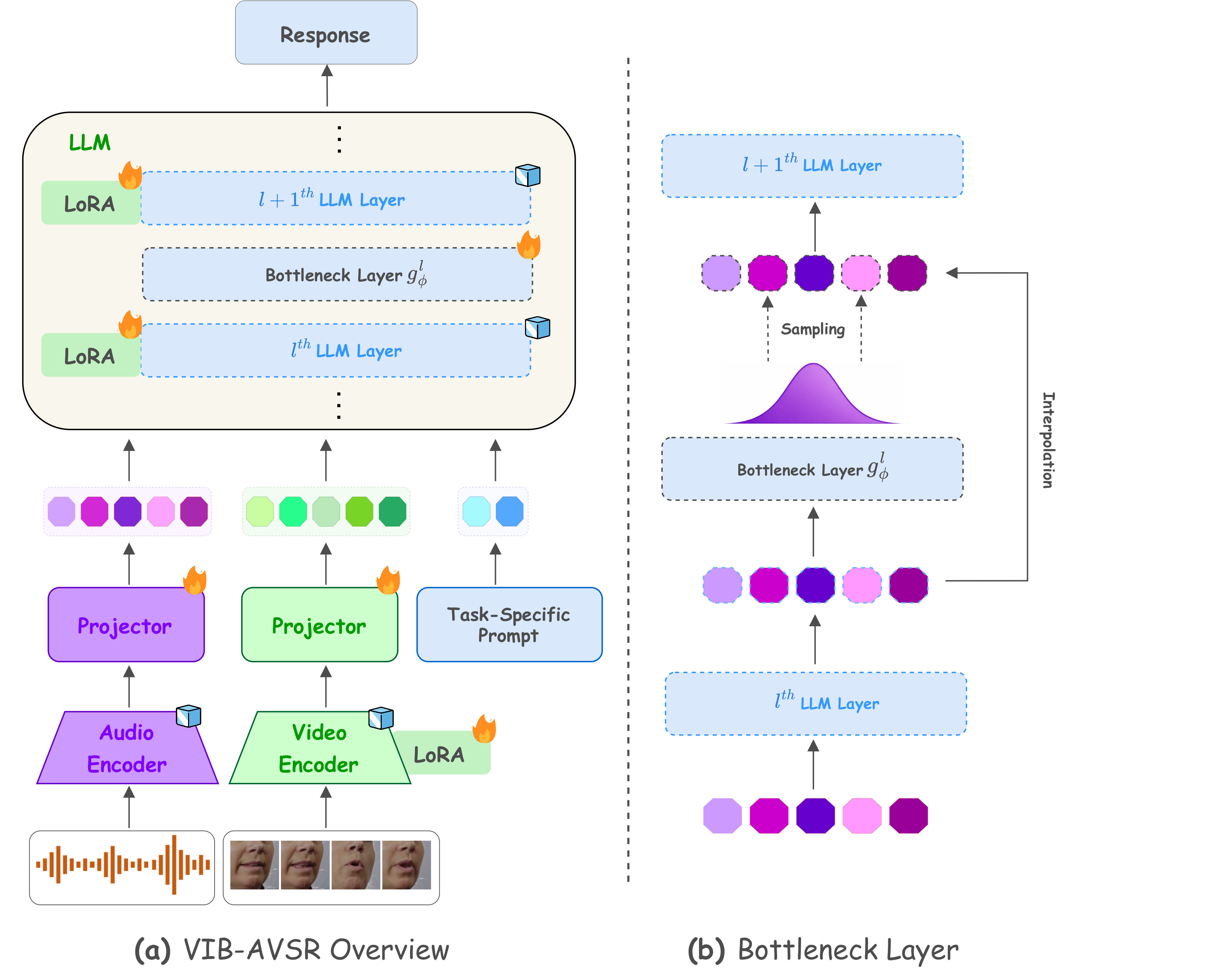
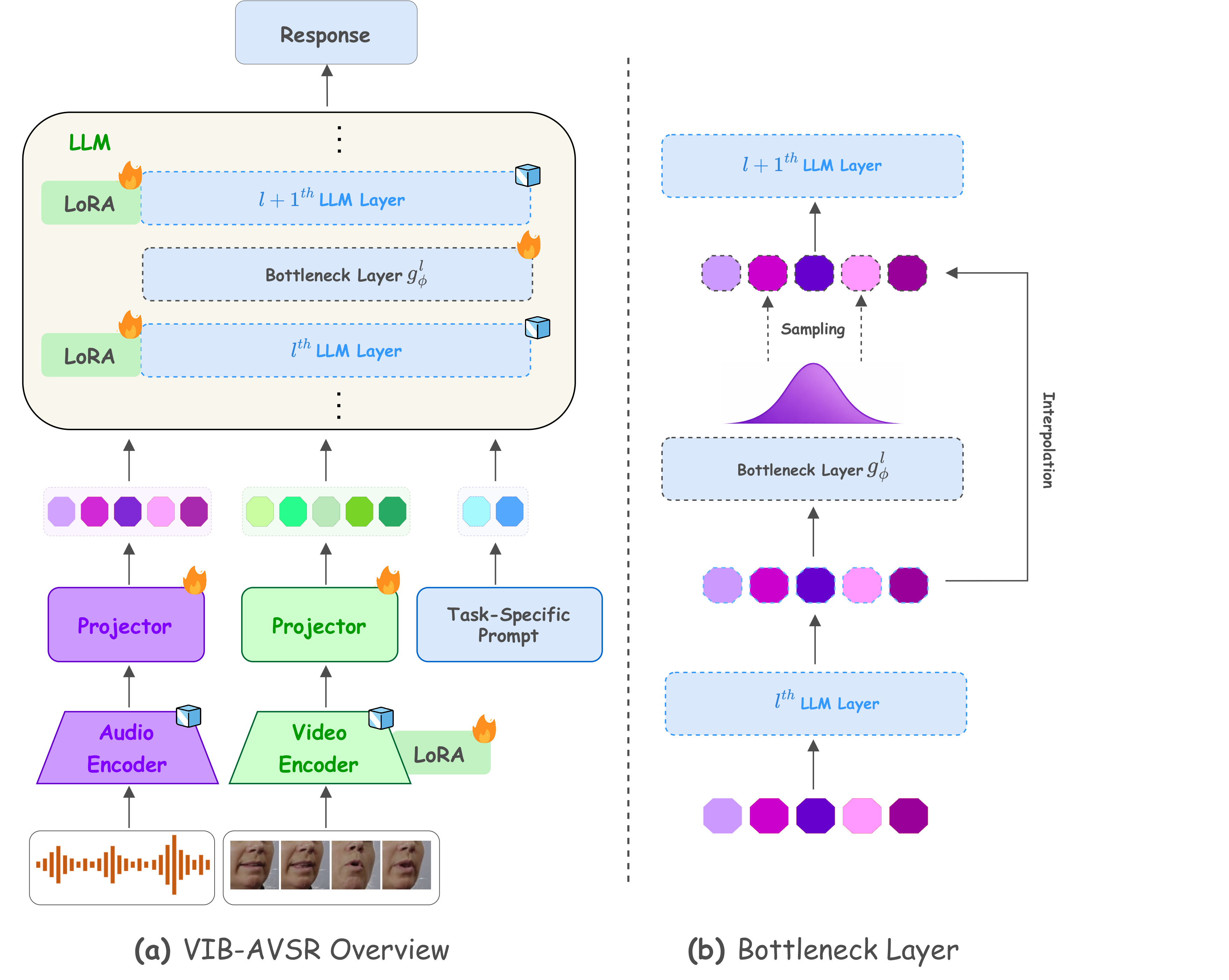
Improves noise robustness in LLM-based audio-visual speech recognition by adding Variational Information Bottleneck layers to compress audio representations and discard noise variance. Achieves significant gains across noise conditions without architectural changes or additional training data.
Links
Abstract
Audio-Visual Speech Recognition takes two input modalities, acoustic and visual streams, where visual information from lip movements aids recognition when audio is noisy. Recently, LLM-based AVSR models have emerged as a promising paradigm by connecting pre-trained audio-visual encoders to an LLM, achieving strong results in clean conditions. However, these models are predominantly optimized for clean acoustic conditions, with limited attention to making the LLM backbone robust to noise. No explicit mechanism is employed to produce stable representations under corrupted audio, leading to performance degradation in noisy environments. To address this, we propose VIB-AVSR, which integrates Variational Information Bottleneck layers at targeted positions within the LLM backbone to regularize representations. VIB-AVSR reduces degradation under noisy conditions across multiple SNR levels and noise types, without requiring architectural modifications or additional training data.
Introduction and Motivation
Audio-Visual Speech Recognition (AVSR) improves transcription by jointly processing acoustic and visual input streams, using lip-movement information to complement the audio signal — especially when audio quality is degraded. The field has advanced considerably through end-to-end deep learning models based on Conformer and Transformer backbones, self-supervised pre-training methods such as AV-HuBERT, and large-scale labeling pipelines such as Auto-AVSR. More recently, approaches that inject visual features into pre-trained speech encoders (e.g., Whisper-Flamingo) have demonstrated strong noise robustness.
The most recent paradigm in AVSR connects pre-trained audio and video encoders to a Large Language Model (LLM) via lightweight adapters, achieving state-of-the-art results. However, noise robustness remains a largely overlooked problem within this LLM-based AVSR paradigm. These models are predominantly optimized for clean acoustic conditions: prior work has documented a significant performance gap when they are tested under noise. This is in stark contrast to traditional encoder-decoder AVSR models trained end-to-end, which can develop noise-robust representations throughout their full architecture.
In LLM-based AVSR, the backbone is a pre-trained language model optimized purely on text — it has never seen noisy audio-visual speech, and only a small subset of its parameters are updated during fine-tuning via LoRA. As a result, no explicit mechanism exists within the LLM backbone to produce stable representations under corrupted audio. The burden of noise robustness falls entirely on the encoders, leaving the LLM itself ill-equipped to handle acoustic domain shift. The authors argue that addressing this requires a principled approach to regularizing the LLM's internal representations directly, rather than relying solely on data augmentation or encoder-only modifications.
Proposed Method: VIB-AVSR
VIB-AVSR integrates Variational Information Bottleneck (VIB) layers at targeted positions within the LLM backbone of a Llama-AVSR-style model. The key idea is to apply information-theoretic compression to the audio hidden states inside the LLM, forcing them to encode only information that is maximally predictive of the transcription target while discarding noise-induced variance. Crucially, VIB-AVSR requires no major architectural changes, no additional training data, and introduces negligible computational overhead.
Base Architecture: Llama-AVSR
The backbone system is Llama-AVSR, a Multimodal Large Language Model for audio-visual speech recognition consisting of three components: (1) modality-specific pre-trained encoders, (2) lightweight linear projectors, and (3) a pre-trained LLM backbone. An audio encoder and a video encoder independently process their input streams, producing feature sequences that are downsampled and projected into the LLM's embedding space. The resulting audio tokens $\mathbf{H}_a$, video tokens $\mathbf{H}_v$, and text tokens $\mathbf{H}_t$ are concatenated and processed by the LLM, which generates transcriptions auto-regressively.
The model is trained with a standard autoregressive objective:
$$\arg\min_\theta \; \mathbb{E}_{X,Y} \left[ \sum_{m=1}^{M} -\log f_\theta(Y_m \mid X^a, X^v, X^t, Y_{Information Bottleneck Principle
The Information Bottleneck (IB) principle (Tishby et al.) provides a framework for learning representations that retain task-relevant information while discarding redundant variation. For an input $X$, a learned representation $Z$ parameterized by $\phi$, and a target $Y$, the IB objective is:
$$\max_{\phi} \; I(Z; Y) - \beta \, I(Z; X)$$where $I(\cdot;\cdot)$ denotes mutual information and $\beta \geq 0$ controls the compression–prediction trade-off. Maximizing $I(Z; Y)$ preserves information predictive of the output, while minimizing $I(Z; X)$ discards redundancy — such as acoustic noise. In the AVSR setting, noise corrupts the audio input $X^a$, causing audio hidden states $\mathbf{H}_a$ to encode noise-specific features. The authors apply the IB objective selectively to $\mathbf{H}_a$, leaving video tokens $\mathbf{H}_v$ and text tokens $\mathbf{H}_t$ unaffected, since they are not directly corrupted by acoustic noise.
Variational Formulation
Direct optimization of the IB objective is intractable due to difficulty estimating mutual information in high-dimensional spaces. Following the variational formulation, the authors derive a tractable lower bound tailored to audio hidden states. The audio encoder and projector produce initial audio representations $\mathbf{H}^0_a$, which are passed into the LLM. Let $\mathbf{H}^l_a \in \mathbb{R}^{T \times d}$ denote the audio hidden states at the output of LLM layer $l$, where $T$ is the number of audio tokens and $d$ is the hidden dimension. A VIB module $g_\phi^l$ takes $\mathbf{H}^l_a$ as input and produces a compressed representation $Z^l_a$.
For the compression term $I(Z^l_a; \mathbf{H}^l_a)$, a factorizable variational prior $r(Z^l_a)$ is introduced and the non-negativity of KL divergence is applied:
$$I(Z^l_a;\, \mathbf{H}^l_a) \;\leq\; \mathbb{E}_{\mathbf{H}^l_a} \left[ D_{\mathrm{KL}}\!\left( p(Z^l_a \mid \mathbf{H}^l_a) \;\|\; r(Z^l_a) \right) \right]$$For the predictive term $I(Z^l_a; Y)$, the true posterior $p(Y \mid Z^l_a)$ is approximated by a variational approximation $q_\phi(Y \mid Z^l_a, X^v, X^t)$, parameterized by the LLM decoder. Omitting the constant $H(Y)$ with respect to model parameters:
$$I(Z^l_a;\, Y) \;\geq\; \mathbb{E}_{X,Y} \left[ \mathbb{E}_{Z^l_a \mid \mathbf{H}^l_a} \left[ \log q_\phi(Y \mid Z^l_a, X^v, X^t) \right] \right]$$Combining both bounds gives the variational IB objective at layer $l$:
$$\mathcal{L}^l_{\mathrm{VIB}} = \mathbb{E}_{X,Y} \left[ \mathbb{E}_{Z^l_a \mid \mathbf{H}^l_a} \left[ \log q_\phi(Y \mid Z^l_a, X^v, X^t) \right] \right] - \beta \, \mathbb{E}_{\mathbf{H}^l_a} \left[ D_{\mathrm{KL}}\!\left( p(Z^l_a \mid \mathbf{H}^l_a) \;\|\; r(Z^l_a) \right) \right]$$The first term is the autoregressive transcription likelihood and the second term regularizes the audio hidden states by penalizing deviation from the prior. $\beta$ controls the compression–prediction trade-off.
Practical Implementation
Using a Monte Carlo approximation and converting to a minimization objective over a mini-batch of $N$ samples:
$$\mathcal{L}_\beta = \frac{1}{N} \sum_{i=1}^{N} \left[ \mathbb{E}_{Z^{l,i}_a \mid H^{l,i}_a} \left[ -\log q_\phi\!\left(Y^i \mid Z^{l,i}_a, X^{v,i}, X^{t,i}\right) \right] + \beta \, D_{\mathrm{KL}}\!\left( p\!\left(Z^{l,i}_a \mid H^{l,i}_a\right) \;\|\; r\!\left(Z^{l}_a\right) \right) \right]$$Both the posterior and prior are modeled as diagonal Gaussians.
Prior distribution. The prior is a learnable diagonal Gaussian:
$$r(Z^l_a) = \mathcal{N}\!\left(Z^l_a;\; \mu^l_r,\; (\sigma^l_r)^2 \cdot I\right)$$where $\mu^l_r \in \mathbb{R}^d$ and $\sigma^l_r \in \mathbb{R}^d_+$ are per-layer parameters shared across all samples, admitting a closed-form KL divergence.
Posterior distribution. The posterior is parameterized by a position-wise two-layer MLP $g_\phi: \mathbb{R}^d \rightarrow \mathbb{R}^{2d}$, applied independently to each audio token embedding — analogous to the feed-forward sublayer of a Transformer. The posterior is:
$$p(Z^l_a \mid \mathbf{H}^l_a) := \mathcal{N}(Z^l_a;\; \mu^l,\; (\sigma^l)^2 \cdot I)$$where $[\mu^l, (\sigma^l)^2] = g_\phi(\mathbf{H}^l_a)$, with mean and variance partitioned along the output dimension. The MLP is applied exclusively to audio token positions, leaving visual and text representations unchanged. Samples are drawn via the reparameterization trick:
$$\tilde{Z}^l_a = \mu^l + \sigma^l \odot \epsilon, \quad \epsilon \sim \mathcal{N}(\mathbf{0}, I)$$At inference, only $\mu^l$ is used (no sampling). To balance compression with the retention of speech-discriminative content, the bottleneck output is interpolated with the pre-bottleneck representation:
$$\hat{Z}^l_a = \alpha \, \mathbf{H}^l_a + (1 - \alpha) \, \tilde{Z}^l_a$$where $\alpha = 0.5$ is fixed for all main experiments. The interpolated representation $\hat{Z}^l_a$ replaces $\mathbf{H}^l_a$ and is propagated to all subsequent LLM layers. In practice, VIB modules are inserted after multiple LLM layers, each with its own independent prior.
Experimental Setup
Dataset
All training and evaluation is conducted on the LRS2 dataset, consisting of BBC program clips with transcribed English speech.
Model Architecture
Following Llama-AVSR, the system uses:
- Audio encoder: Whisper-medium (frozen throughout training)
- Video encoder: AV-HuBERT (fine-tuned with LoRA, rank 16)
- LLM backbone: Llama-3.2-1B (fine-tuned with LoRA, rank 64)
- Projectors: Modality-specific linear projectors mapping encoder features to the LLM embedding space
- Token compression rate: 3× for both audio and video tokens
VIB modules are inserted after selected LLM layers and trained jointly with the LoRA modules. Each VIB module $g_\phi^l$ is a two-layer MLP: a linear layer followed by GeLU activation and a second linear layer with $2H$ output neurons, from which mean and log-variance of the variational posterior are obtained. The same model configuration is used for both Llama-AVSR and VIB-AVSR for fair comparison.
Training Paradigms
Two training paradigms are evaluated:
- Clean Paradigm: No noise is added to audio during training. This tests whether the VIB regularization generalizes to noisy test conditions even without noise augmentation.
- Noisy Paradigm: A random noise type is added to training audio with SNR level sampled uniformly at random per instance. This evaluates whether VIB further improves robustness on top of noise augmentation.
Evaluation Protocol
Word Error Rate (WER) is reported under two noise types — babble and speech noise — sampled from the MUSAN dataset at five SNR levels: $-10$, $-5$, $-2$, $0$, $5$ dB, plus a noise-free condition ($\infty$ dB). The metric Avg ($N > S$) is introduced as the average WER over extreme noise conditions ($-10$, $-5$, $-2$ dB), where noise dominates the signal.
Main Results
The table below summarizes WER for Llama-AVSR and VIB-AVSR across both noise types and training paradigms.
| Training | Method | Babble SNR (dB): −10 / −5 / −2 / 0 / 5 | Babble Avg | Babble Avg (N>S) | Speech SNR (dB): −10 / −5 / −2 / 0 / 5 | Speech Avg | Speech Avg (N>S) | ∞ | ||||||||
|---|---|---|---|---|---|---|---|---|---|---|---|---|---|---|---|---|
| Noisy | Llama-AVSR | 34.87 | 27.55 | 18.09 | 8.00 | 5.74 | 18.85 | 26.84 | 27.66 | 14.94 | 9.14 | 5.21 | 3.84 | 12.16 | 17.24 | 2.72 |
| VIB-AVSR | 32.52 | 25.63 | 15.63 | 7.82 | 5.35 | 17.39 | 24.59 | 27.52 | 13.23 | 8.90 | 5.08 | 3.98 | 11.74 | 16.55 | 2.38 | |
| Clean | Llama-AVSR | 47.03 | 34.32 | 20.20 | 8.61 | 5.19 | 23.07 | 33.85 | 42.13 | 18.44 | 10.78 | 5.30 | 4.32 | 16.20 | 23.78 | 2.34 |
| VIB-AVSR | 40.97 | 31.50 | 19.45 | 8.55 | 5.00 | 21.09 | 30.64 | 37.44 | 17.37 | 10.69 | 5.36 | 4.39 | 15.05 | 21.83 | 2.42 | |
Noisy Training
Under noisy training, VIB-AVSR almost always reduces WER relative to Llama-AVSR, with the largest gains at lower SNRs — particularly under babble noise. The average WER under babble noise improves from 18.85% to 17.39%, and the extreme-noise average (Avg $N > S$) improves from 26.84% to 24.59%. Under speech noise, improvements are smaller but VIB-AVSR still reduces WER across all conditions except 5 dB. Critically, VIB-AVSR also achieves lower WER under noise-free evaluation ($\infty$: 2.38% vs. 2.72%), indicating that the bottleneck acts as an effective regularizer even beyond the noisy conditions themselves.
Clean Training
When trained without any noise augmentation, VIB-AVSR still yields substantial WER reductions at test time. Under babble noise, improvements appear across all SNR levels. The babble average WER drops from 23.07% to 21.09%, and the extreme-noise average from 33.85% to 30.64%. Under speech noise, consistent gains appear in the low-SNR regime. Notably, the bottleneck is never exposed to noisy samples during training, yet the learned representations generalize more effectively to unseen noisy conditions. This suggests that variational compression promotes robustness through a mechanism fundamentally distinct from data augmentation. Models trained on clean data degrade more sharply under extreme noise than noisy-trained counterparts, but VIB-AVSR consistently narrows this gap relative to Llama-AVSR, particularly at the lowest SNRs. Performance on clean speech ($\infty$) remains comparable (2.42% vs. 2.34%), confirming that robustness gains do not come at the expense of clean-condition performance.
Ablation Studies
Effect of VIB Layer Placement
The placement of VIB modules determines at which depth noise-corrupted representations are compressed. Inserting too early may interfere with low-level features; inserting too late leaves noise unmitigated. The study evaluates single, dual, and triple bottleneck configurations at various layer positions, using noisy training paradigm and $\beta = \frac{0.1}{H}$. Layer index $-1$ denotes placement immediately after the audio encoder (at the projection layer), with $\beta = 10^{-7}$ following prior work; no interpolation is applied here due to shape mismatch.
| Config | Layer(s) | −10 dB | −5 dB | −2 dB | 0 dB | 5 dB | ∞ | Avg |
|---|---|---|---|---|---|---|---|---|
| Single | ||||||||
| −1 | 33.25 | 25.27 | 16.29 | 7.33 | 5.59 | 2.37 | 15.03 | |
| 2 | 34.76 | 25.59 | 16.95 | 7.12 | 5.20 | 2.43 | 15.32 | |
| 4 | 34.73 | 25.50 | 16.95 | 8.17 | 5.18 | 2.61 | 15.52 | |
| 6 | 34.59 | 26.32 | 16.85 | 7.48 | 5.36 | 2.76 | 15.56 | |
| 8 | 34.53 | 26.44 | 17.67 | 7.55 | 5.09 | 2.46 | 15.63 | |
| 12 | 34.29 | 25.92 | 17.66 | 8.59 | 5.39 | 2.31 | 15.69 | |
| Dual | ||||||||
| 2, 6 | 35.11 | 25.93 | 17.76 | 7.48 | 5.62 | 2.70 | 15.77 | |
| ★ Best | 4, 8 | 33.14 | 24.61 | 16.24 | 7.42 | 5.38 | 2.38 | 14.86 |
| 8, 12 | 33.45 | 25.71 | 16.26 | 7.73 | 5.26 | 2.54 | 15.16 | |
| Triple | ||||||||
| −1, 4, 8 | 34.56 | 25.66 | 16.38 | 8.03 | 6.68 | 2.81 | 15.68 | |
| 4, 8, 12 | 33.27 | 26.61 | 17.55 | 7.85 | 6.31 | 2.90 | 15.75 | |
Key findings:
- Single-layer configurations perform comparably across positions, with no single placement offering a consistent advantage. The $-1$ configuration (early compression at the encoder-LLM interface) achieves the best single-layer average WER at 15.03%, but still falls short of the best dual configuration.
- Dual configuration (4, 8) yields the best overall performance, achieving the lowest average WER (14.86%) and the strongest gains under extreme noise, while remaining competitive at higher SNR levels. The advantage of (4, 8) over (8, 12) at low SNR suggests that compressing representations at an earlier intermediate layer is beneficial when noise is most severe.
- Triple configurations degrade performance across all conditions including clean speech, indicating that stacking too many compression stages leads to over-regularization. This motivates the use of dual placement as the default.
Effect of $\beta$
$\beta$ controls the strength of the KL regularization term. Too small a value reduces the regularization effect; too large a value risks discarding task-relevant features. Four values normalized by hidden dimension $H$ are ablated using the (4, 8) dual configuration:
| $\beta / H$ | −10 dB | −5 dB | −2 dB | 0 dB | 5 dB | ∞ | Avg |
|---|---|---|---|---|---|---|---|
| 0.05 | 33.84 | 25.42 | 16.52 | 7.63 | 5.48 | 2.84 | 15.29 |
| 0.1 | 33.14 | 24.61 | 16.24 | 7.42 | 5.38 | 2.38 | 14.86 |
| 0.2 | 34.40 | 24.80 | 16.66 | 7.63 | 5.53 | 2.49 | 15.25 |
| 1 | 35.86 | 27.73 | 19.49 | 10.72 | 8.03 | 4.25 | 17.68 |
At $\beta = 1$, performance degrades sharply across all SNR levels, with average WER rising to 17.68% — confirming that excessive compression is harmful. Among the remaining values, $\beta = 0.1/H$ achieves the best average WER of 14.86% and is the most consistent across conditions, and is therefore used in all other experiments.
Role of Interpolation Coefficient $\alpha$
Three configurations of $\alpha$ are compared using the (4, 8) dual setup with $\beta = 0.1/H$:
| $\alpha$ | −10 dB | −5 dB | −2 dB | 0 dB | 5 dB | ∞ | Avg |
|---|---|---|---|---|---|---|---|
| 0 (fully compressed) | 37.62 | 31.13 | 22.41 | 13.23 | 8.32 | 4.58 | 19.54 |
| $0 \rightarrow 0.5$ (scheduled) | 33.54 | 26.75 | 18.45 | 9.05 | 6.56 | 3.43 | 16.29 |
| 0.5 (fixed) | 33.14 | 24.61 | 16.24 | 7.42 | 5.38 | 2.38 | 14.86 |
- Setting $\alpha = 0$ replaces the hidden state entirely with the sampled representation, leading to the worst performance across all conditions — consistent with over-regularization and excessive information loss.
- The cosine-scheduled variant ($0 \rightarrow 0.5$) improves over $\alpha = 0$ but still shows higher WER relative to the fixed setting. The authors attribute this to the period of near-complete compression early in training, which the LLM must recover from, leaving a lasting negative imprint on learned representations.
- Fixed $\alpha = 0.5$ consistently achieves the best performance and is used for all main experiments.
Summary of Key Design Choices
Based on the ablation studies, the following configuration is identified as most effective and used throughout the main experiments:
- VIB insertion layers: After LLM layers 4 and 8 (dual configuration)
- Regularization strength: $\beta = 0.1 / H$ where $H$ is the LLM hidden dimension
- Interpolation coefficient: $\alpha = 0.5$ (fixed throughout training)
- Inference: Use $\mu^l$ only (no stochastic sampling at test time)
- Audio encoder: Frozen — only projection layers and LoRA are trained alongside the VIB modules
Contributions and Novelty
The paper makes the following contributions:
- Proposes VIB-AVSR, a lightweight method that integrates VIB layers into the LLM backbone of an AVSR model to improve noise robustness at the representation level, without requiring architectural redesign or additional training data.
- Demonstrates that VIB-AVSR improves noise robustness under both noisy and clean training paradigms, showing that variational compression promotes generalization to noisy conditions even without noise augmentation exposure.
- Provides extensive ablation studies on VIB layer placement, regularization strength $\beta$, and interpolation coefficient $\alpha$, with empirical evidence supporting each design choice.
- Shows WER reductions over Llama-AVSR across multiple noise types (babble and speech) and SNR levels, with gains that widen under extreme noise conditions, while preserving recognition performance on clean speech.
Limitations and Discussion
Several limitations and boundary conditions are noted or implied by the results:
- Experiments are conducted exclusively on the LRS2 dataset with Llama-3.2-1B as the LLM backbone. Generalization to other benchmarks (e.g., LRS3, VoxCeleb2) or larger LLMs is not demonstrated in this paper.
- The method is evaluated with babble and speech noise types from MUSAN. Generalizability to other noise types (e.g., music, environmental noise) is not explicitly verified.
- The gains under speech noise are smaller than those under babble noise. Speech noise is spectrally similar to the target signal, making it harder to compress away with the information bottleneck.
- Adding a third VIB module leads to over-regularization and degraded performance, suggesting that the benefit of the bottleneck saturates quickly and that careful placement with limited depth is important.
- The approach requires careful selection of $\beta$ and $\alpha$ through ablation, which may require additional tuning effort when adapting to new architectures or datasets.
- The clean-condition performance under clean training is marginally higher for Llama-AVSR (2.34% vs. 2.42%), indicating a small trade-off when no noise is seen during training — though this is within a very small absolute margin.
Conclusion
VIB-AVSR introduces a principled, lightweight approach to improving noise robustness in LLM-based audio-visual speech recognition. By inserting Variational Information Bottleneck modules into intermediate layers of the LLM backbone — specifically after layers 4 and 8 in a Llama-3.2-1B backbone — and applying variational compression exclusively to audio token representations, the model is encouraged to retain acoustically relevant content while discarding noise-correlated features. The method requires no architectural redesign, no additional training data, and introduces negligible computational overhead.
Experiments under babble and speech noise show consistent WER reductions over the Llama-AVSR baseline across SNR levels and training paradigms. Notably, the gains hold even when no noise augmentation is used during training, demonstrating that variational compression promotes noise-robust representations through a mechanism fundamentally distinct from data augmentation. The gains are largest under extreme noise conditions (SNR $\leq -2$ dB), precisely where robust acoustic representations matter most for practical deployment of conversational and audio-visual AI systems.
Code & Implementation
This repository is a placeholder. At the time of review, the GitHub repository contains only a README file stating the code is "official," but no source code has been released. The actual implementation of VIB-AVSR—including the Variational Information Bottleneck layer integration, LLM backbone modifications, and training/evaluation scripts—is marked as pending.
Once published, the repository is expected to contain:
- VIB layer implementations for the LLM backbone
- Audio-visual encoder integration with LLM
- Training and evaluation scripts for noisy audio-visual speech recognition
- Baseline model definitions and experimental configurations